What to Train on Telemetry

By Alexander Chernov. First published on LinkedIn, 2026-10-12. Read the original.

Part 3 of three on machine and user telemetry. Part 1 was the pipeline, Part 2 was how much of the data to keep, and this part is what to train on it.

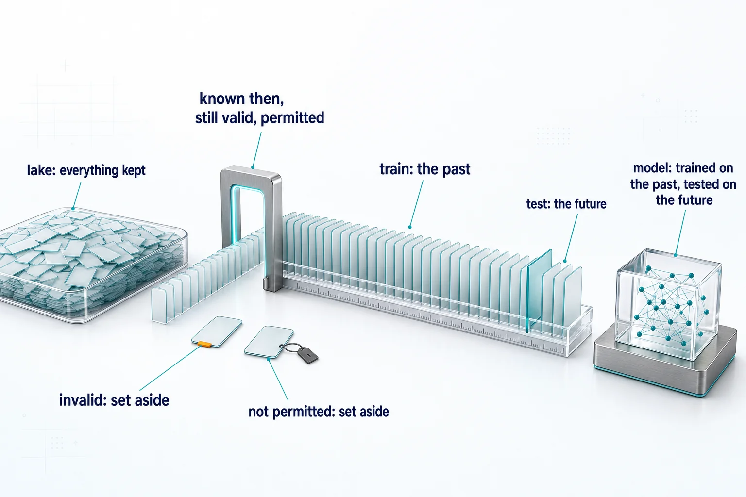
A training set is not everything the lake holds. It is the part that was known at the time of each prediction, is still valid, and is permitted for training. The same few kinds of model serve machines and users, from failure risk to next-step suggestions, and in both cases the way that training set is built matters more than the choice of algorithm.

Five rules build it. Compute every feature as it was known when the prediction would have been made. Split by time, and keep each training window inside the validity windows from Part 2. Where outcomes arrive slowly, predict earlier proxy targets and check them against the outcomes as they arrive. Account for how the data was sampled. Treat training as an operation the dataset must permit.

Part 1 built one pipeline for machine and user telemetry, and Part 2 decided what it keeps and for how long. Each record now carries its versions, a validity window and its policy. Training is where those fields matter most, because a model learns every relationship in its training set, including the ones that no longer hold. For equipment, the examples come from the estate in my two articles on 100,000 devices: bioreactors, chromatography skids, analytical instruments and sequencers on one streaming platform.

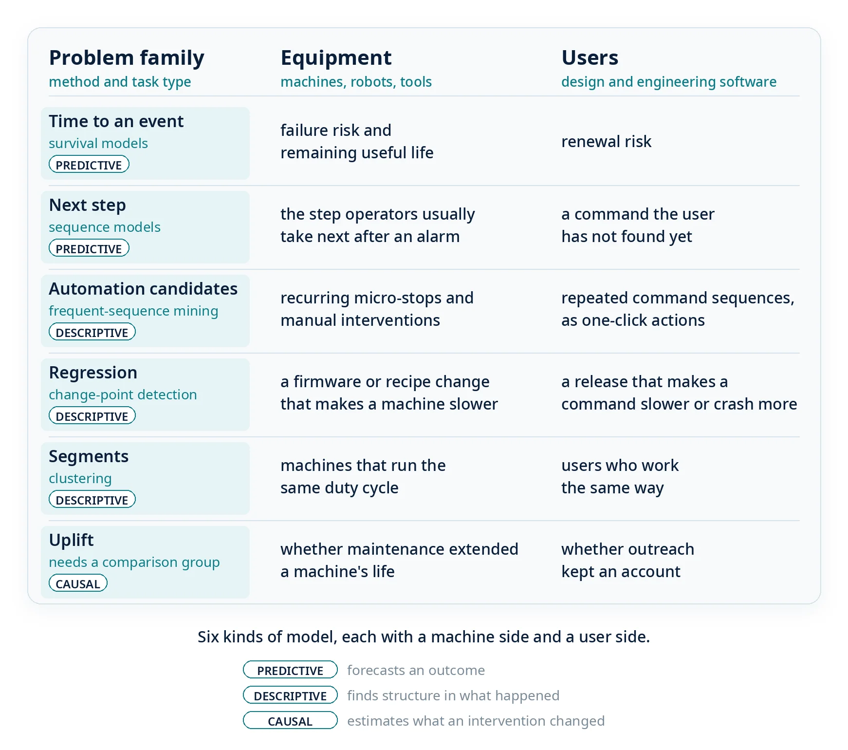
Six kinds of model, each with a machine side and a user side

Failure risk and remaining useful life on the equipment side have a counterpart in renewal risk on the user side. Both ask how long until an event, and survival models answer that well. Most machines have not failed yet and most accounts have not lapsed. A survival model counts each of them as what it is, a unit that has lasted at least this long, instead of dropping it or treating it as one that never fails. Gradient-boosted classifiers with calibrated probabilities are the common alternative when a fixed horizon, such as the next 30 days, is enough.

The next operator action and the next command are the same kind of problem: predicting the next step in a sequence. The vocabulary of steps and the cost of a wrong suggestion differ between the two. Collaborative filtering over who did what is the simple start, and a sequence model over sessions is the stronger one. On a line it suggests the step operators usually take next after an alarm. In a design tool it suggests a command the user has not found yet.

Recurring micro-stops and manual interventions on a line are candidates for automation, and repeated command sequences in a product are candidates for one-click assistant actions. Frequent-sequence mining finds both, ranked by how often a sequence occurs times how long it takes.

A firmware or recipe change that makes a machine slower or noisier is the counterpart of a release that makes a command slower or crash more often. Change-point and anomaly detection on per-version metrics find both, and the envelope from Part 1 already carries the versions to split by. In the 100,000-device articles, one analytical instrument was modeled with a firmware defect that made it publish 20,000 events a second instead of 10. A detector on per-version event rates exists to catch exactly that.

Fleet segments and user segments come from clustering usage: machines that run the same duty cycle, users who work the same way.

The last pair asks whether an intervention helped: whether maintenance extended a machine’s life, whether outreach kept an account. That is uplift modeling, and it is a causal question. It needs a comparison group that did not receive the intervention. A randomized holdout is the strongest design where withholding the intervention is safe and acceptable, as it usually is for outreach. Preventive maintenance on a high-risk machine usually cannot be withheld, so the comparison comes from a staggered rollout or an adjusted observational cohort, with the assumptions behind it stated, and the causal reading is weaker. Without a comparison group, the model learns which machines were chosen for maintenance, not what the maintenance did.

Features as they were known at prediction time

Every feature is computed as it was when the prediction would have been made. A model that sees a value from after that moment learns something it will never have in production. The common leaks sit close to the label: a work order written after a failure, or a cancellation-flow event recorded once a user has already decided to leave.

A value has two times, not one: the time it describes and the time it became known. A sensor’s readings may be corrected backward after a recalibration, and sessions are rebuilt when a definition changes. A training row should see each value as it was known at prediction time, not as corrected later.

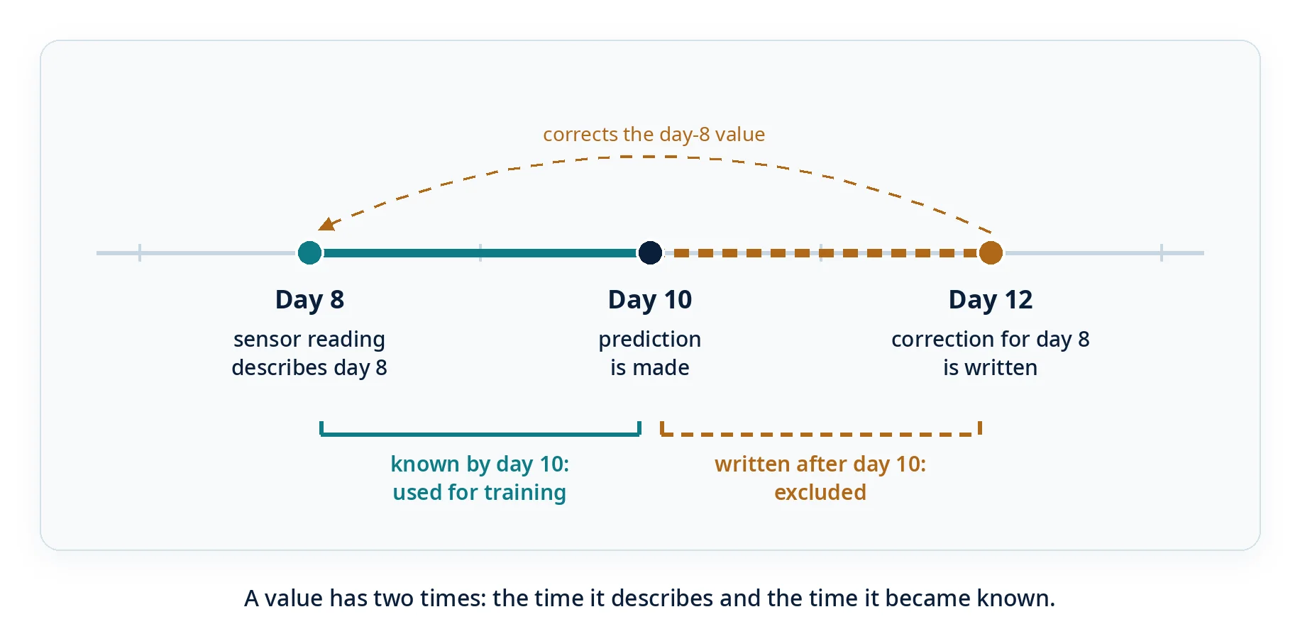
At 100,000 devices the second time is routine. When a site of 12,000 devices loses its link for twenty minutes, the devices buffer and replay on reconnection, so every buffered reading describes a moment during the outage but becomes known only after it. A prediction made during the outage could not have seen those readings, and its training row must not either. The earlier articles ended on whether the exact state of a batch can be reconstructed at a point in time. A training row asks the same question about the moment of each prediction.

Feature stores do point-in-time joins for this, and the detail matters. Feast, by default, constrains only the time a value describes, so a value backfilled or corrected afterward can still reach the training set unless the time it was written is also used. Its filter_by_created_timestamp option adds that second condition on the offline stores that support it, and the others raise an error rather than ignore it.

The features come from the metric layer of Part 1. The dashboard, the model and the agent then compute cycle time or retention the same way.

The three data planes from the 100,000-device articles map onto a training set. Operational events such as AlarmRaised or QualityCheckFailed supply the labels, the telemetry plane supplies the features, and bulk data such as spectra and images stays in object storage, reached through the pointer its event carries.

Split by time, inside the validity windows

Training sets are split by time, not at random: train on the past, test on the future. Telemetry is autocorrelated, and a random split puts near-copies of the test rows into training, which makes a model look better than it will be. Splitting by machine or by user as well keeps one unit’s behavior from appearing on both sides.

Evaluation follows the rule of the 100,000-device articles: nothing fails at the average. A model scored across the whole fleet is scored mostly on the devices that report most and fail least, so it is evaluated per equipment class, per site and per segment.

Part 2 gave every record a validity window, and the training set respects it. A window that spans a recalibration, a recipe or firmware change, or a metric redefinition teaches the model a relationship that no longer holds. There are three ways across such a change. Train only inside the current window. Carry the version as a feature, so the model can tell the regimes apart. Or rebuild the history under the current definition by replay from the lake, as Part 1 described. Which one fits depends on how much data the current window holds.

Erasure and withdrawn consent, which Part 2 also counted as validity events, reach the training set through its snapshot. Each run builds its set from a snapshot of the lake and records the revision it used, as the Agentic Datasets assertion cited in Part 2 requires of every result. Experiment trackers such as MLflow log the dataset and a digest beside the run.

That record names the input, not its rows, and Part 2’s snapshots expire. So each run also keeps its training snapshot, or an index of the records in it, for as long as its model is in use. A withdrawn record is then left out of every future set, and each earlier model that saw it can be found and assessed for retraining or retirement.

Proxy targets for slow outcomes

Some outcomes take a long time to arrive. A renewal happens once a year, and a failure may happen once in the life of a machine. Waiting for them leaves too few examples, too late.

The workable approach is to predict an earlier proxy target, such as 30 days of inactivity for an account or a rising vibration band for a bearing. A proxy is not the outcome. Inactivity is not non-renewal and vibration is not failure, so the two are kept as separate labels. As confirmed outcomes come in, they become the ground truth the proxy is checked against. A proxy that stops predicting its outcome is retired, like any metric that no longer informs a decision.

Account for how the data was sampled

Every decision in Part 2 shapes a training set. Full command sequences were kept for a hashed sample of sessions. The inclusion rule is known, so models trained on them can carry sample weights that restore the population.

High-rate waveforms were captured only in a window around a fault, so a waveform set is almost all faults. A model trained on it sees failure far more often than failure happens. Weights cannot repair that on their own, because the normal stretches were never recorded. The model needs normal windows captured on purpose, then weighted to their real share.

In the illustrative estate of the 100,000-device articles, five percent of the devices produce nearly two thirds of the events. A training set drawn per event learns those devices, not the fleet, and one faulty instrument would fill it. So examples are drawn or weighted per device, as Part 2 counted independent units rather than events.

The hot store holds about a week of data and is not a training source at all.

Training is a use the data must permit

Whether a dataset may be trained on depends on where it came from, the policy attached to it, its quality, whether it is still valid, and whether it represents the population the model will serve. That is decided per dataset, before the run.

On the equipment side, the question is often contractual: telemetry from a customer’s plant is covered by an agreement that may or may not include training a model. On the user side, it is the purpose users were told about when the data was collected.

Croissant 1.1, the MLCommons metadata format for machine-learning datasets, can now write conditions of use into a dataset’s description. My public Croissant policy profile adds the part that decides them. A dataset declares the operations it admits and the conditions for each, and a gate refuses any operation the dataset does not declare. Training is one operation among the others, so data collected for support or for a batch record is refused for training until its description admits it.

The description does not create the right. It records what the contract, the consent and the law already allow, and the gate enforces that record. A description that admits training without them behind it is a defect, not a permission.

This extends the chain from Part 1. Access rules and lineage followed the data from event to session to metric to agent tool. They now continue to the training set and the model.

Scores reach agents through the metric layer

Most of these models are best served in batch. Daily scores are written into the metric layer, where the dashboards and agents of Part 1 already read. Suggestions are precomputed into an online store.

A real-time endpoint is worth having only where the session context matters, such as the next command in an open session. A provisioned endpoint bills for every hour it is up, called or not, while a batch job bills only while it runs. So the rule is to precompute wherever the session context is not needed.

Agents read scores through the same governed tools as metrics, served through the Model Context Protocol. A maintenance agent reads a machine’s failure risk with the features that contributed most to it, computed with SHAP. SHAP says which inputs moved the score, not what caused the failure. A customer-success agent reads an account’s renewal risk the same way, and the in-product assistant reads next-command and repetition candidates. Every action an agent takes on a score leaves a decision record.

The loop changes its own labels

Outcomes return to the lake as the next round’s labels, and here the models affect their own data. A machine maintained because its risk score was high does not fail, and an account contacted because it looked at risk may renew. Trained naively on those outcomes, the next model learns that high-risk machines do not fail. The absence of a failure after maintenance is not evidence that the risk score was wrong.

Where withholding the intervention is safe, a randomized holdout keeps a clean signal and doubles as the uplift model’s comparison group. Where it is not, as for a high-risk machine, the comparison designs from the uplift paragraph apply, with their assumptions stated. The decision records say which units were acted on, so the next training set can tell treated units from untreated ones.

Drift checks compare live features and scores with the training data. Part 2’s validity events, such as a recalibration, a release or a metric redefinition, are known causes of drift. Each one can open a retraining review directly, without waiting for a drift check to notice.

The techniques here are established ones: point-in-time joins, time-based splits, survival models, sampling adjustments, holdouts and uplift. What the series adds is that the versions, validity windows and use permissions that govern telemetry and agent actions also govern the data a model is trained on.

Sources. One Pipeline for Machines and People (Part 1): https://www.linkedin.com/pulse/one-pipeline-machines-people-alexander-chernov-dn9qc/ · How Much Telemetry Is Enough (Part 2): https://www.linkedin.com/pulse/how-much-telemetry-enough-alexander-chernov-n3xnc/ · At 100,000 Devices, Throughput Is the Easy Part: https://www.linkedin.com/pulse/100000-devices-throughput-easy-part-alexander-chernov-tz7bc/ · At 100,000 Devices, Nothing Fails at the Average: https://www.linkedin.com/pulse/100000-devices-nothing-fails-average-alexander-chernov-cdcec/ · Feast, point-in-time joins: https://docs.feast.dev/getting-started/concepts/point-in-time-joins · scikit-learn, cross-validation of time series data: https://scikit-learn.org/stable/modules/cross_validation.html · lifelines, introduction to survival analysis and censoring: https://lifelines.readthedocs.io/en/latest/Survival%20Analysis%20intro.html · Gutierrez and Gérardy, Causal Inference and Uplift Modelling: A Review of the Literature, PMLR 67 (2017): https://proceedings.mlr.press/v67/gutierrez17a.html · Lundberg and Lee, A Unified Approach to Interpreting Model Predictions, NeurIPS 2017: https://papers.nips.cc/paper/7062-a-unified-approach-to-interpreting-model-predictions · MLflow dataset tracking: https://mlflow.org/docs/latest/ml/dataset/ · Agentic Datasets conformance assertions: https://github.com/agentic-datasets/reference/blob/main/CONFORMANCE.md · Croissant 1.1 specification, data use conditions: https://docs.mlcommons.org/croissant/docs/croissant-spec-1.1.html · Croissant policy profile: https://github.com/doytsujin/ok-croissant-policy-profile · Croissant policy profile, archived release: https://doi.org/10.5281/zenodo.22018156 · Model Context Protocol specification: https://modelcontextprotocol.io/specification

#MachineLearning #MLOps #DataEngineering #IndustrialIoT #Telemetry #PredictiveMaintenance #FeatureStore #DataGovernance #AgenticAI

Keyboard shortcuts

Articles